In the rapidly evolving world of market research, understanding consumer sentiments and preferences is crucial for developing effective marketing strategies and successful products. Our client, a leading market research firm, sought to harness the power of Speech Emotion Recognition (SER) to gain deeper insights into customer emotions. By analyzing extensive audio data from customer surveys and focus groups, the firm aimed to uncover valuable emotional trends that could inform its strategic decisions. This technical blog post details the implementation of an SER system, highlighting the challenges, approach, and impact.

Building an effective Speech Emotion Recognition (SER) system involves primary challenges revolving around several key areas. 

• Predicting the user’s emotion accurately based on spoken utterances is inherently complex due to the subtle and often ambiguous nature of emotional expressions in speech. 
• Achieving high accuracy in recognizing and classifying these emotions from speech signals is crucial but challenging, as it requires the model to effectively distinguish between similar emotions. 
• Another significant challenge is bias mitigation, ensuring the system performs well across different emotions and does not disproportionately favor or overlook specific ones. 
• Contextual understanding is also essential, as emotions are often influenced by the broader context of the conversation, requiring the system to consider previous utterances or dialogues to refine its emotional understanding, adding another layer of complexity to the model’s development. 

Addressing these core challenges is crucial for creating a robust and reliable SER system that can provide valuable insights from audio data.

Speech Emotion Recognition (SER) involves detecting and interpreting human emotions from spoken audio signals. This process combines principles from audio signal processing, feature extraction, and machine learning. Accurately capturing and classifying the nuances of speech that convey different emotions, such as tone, pitch, and intensity, is key to SER. Commonly used features include Mel-Frequency Cepstral Coefficients (MFCC), Chroma, Mel Spectrogram, and Spectral Contrast, representing the audio signal in a machine-readable format.

We have referred to the Speech Emotion Recognition Kaggle Notebook for the project.

We began by gathering four diverse datasets to ensure a comprehensive range of emotional expressions: 

• The Ryerson Audio-Visual Database of Emotional Speech and Song (RAVDESS), 
• Crowd-Sourced Emotional Multimodal Actors Dataset (CREMA-D), 
• Surrey Audio-Visual Expressed Emotion (SAVEE), and 
• Toronto Emotional Speech Set (TESS). 

Each audio file was converted to a consistent WAV format and resampled to a uniform sampling rate of 22050 Hz to ensure uniformity across the dataset. This preprocessing step is crucial as it standardizes the input data, making it easier for the model to learn the relevant features.

Feature Extraction

Feature extraction transforms raw audio data into a format suitable for machine learning algorithms. Using the Librosa library, we extracted several key features:

• Mel-Frequency Cepstral Coefficients (MFCC): Capturing the power spectrum of the audio signal, we extracted 40 MFCC coefficients for each audio file.
• Chroma: This feature represents the 12 different pitch classes, providing harmonic content information.
• Mel Spectrogram: A spectrogram where frequencies are converted to the Mel scale, aligning closely with human auditory perception, using 128 Mel bands.
• Spectral Contrast: Measuring the difference in amplitude between peaks and valleys in a sound spectrum, capturing the timbral texture.

Data Augmentation

We applied several data augmentation techniques to enhance the model’s robustness and generalizability, including noise addition, pitch shifting, and time-stretching. Introducing random noise simulates real-world conditions, modifying the pitch accounts for variations in speech, and altering the speed of the audio without changing the pitch introduces variability. These techniques increased the dataset’s variability, improving the model’s ability to generalize to new, unseen data.

Data Splitting

The dataset was divided into training, validation, and test sets, with a common split ratio of 70% for training, 20% for validation, and 10% for testing. This splitting ensures that the model is trained on one set of data, validated on another, and tested on a separate set to evaluate its performance objectively.

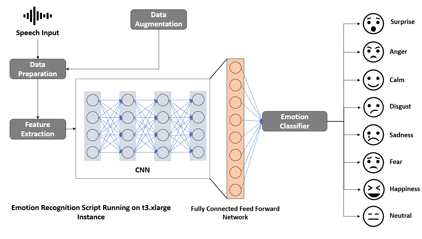
Model Building

We chose Convolutional Neural Networks (CNNs) for their effectiveness in capturing spatial patterns in audio features. The model architecture included multiple layers, each configured to extract and process features progressively:

1. Input Layer Configuration

The first step in model building is defining the input layer. The input shape corresponds to the extracted features from the audio data. For instance, when using Mel-Frequency Cepstral Coefficients (MFCCs), the shape might be (40, 173, 1), where 40 represents the number of MFCC coefficients, 173 is the number of frames, and 1 is the channel dimension.

2. Convolutional Layers

Convolutional Neural Networks (CNNs) are particularly effective for processing grid-like data such as images or spectrograms. In our SER model, we use multiple convolutional layers to capture spatial patterns in the audio features.

First Convolutional Layer:

Filters: 64

Kernel Size: (3, 3)

Activation: ReLU (Rectified Linear Unit)

This layer applies 64 convolution filters, each of size 3×3, to the input data. The ReLU activation function introduces non-linearity, allowing the network to learn complex patterns.

Second Convolutional Layer:

Filters: 128

Kernel Size: (3, 3)

Activation: ReLU

This layer increases the depth of the network by using 128 filters, enabling the extraction of more detailed features.

3. Pooling Layers

Pooling layers are used to reduce the spatial dimensions of the feature maps, which decreases the computational load and helps prevent overfitting.

MaxPooling:

Pool Size: (2, 2)

MaxPooling layers follow each convolutional layer. They reduce the dimensionality of the feature maps by taking the maximum value in each 2×2 patch of the feature map, thus preserving important features while discarding less significant ones.

4. Dropout Layers

Dropout layers are used to prevent overfitting by randomly setting a fraction of input units to zero at each update during training.

First Dropout Layer:

Rate: 0.25

This layer is added after the first set of convolutional and pooling layers.

Second Dropout Layer:

Rate: 0.5

This layer is added after the second set of convolutional and pooling layers, increasing the dropout rate to further prevent overfitting.

5. Flatten Layer

This layer flattens the 2D output from the convolutional layers to a 1D vector, which is necessary for the subsequent fully connected (dense) layers.

6. Dense Layers

Fully connected (dense) layers are used to combine the features extracted by the convolutional layers and make final classifications.

First Dense Layer:

Units: 256

Activation: ReLU

This dense layer has 256 units and uses ReLU activation to introduce non-linearity.

Second Dense Layer:

Units: 128

Activation: ReLU

This layer further refines the learned features with 128 units and ReLU activation.

7. Output Layer

The output layer is designed to produce the final classification into one of the emotion categories.

Units: Number of emotion classes (e.g., 8 for the RAVDESS dataset)

Activation: Softmax

The softmax activation function is used to output a probability distribution over the emotion classes, allowing the model to make a multi-class classification.

Model Configuration Summary:

• Input Shape: (40, 173, 1)
• First Convolutional Layer: 64 filters, (3, 3) kernel size, ReLU activation
• First MaxPooling Layer: (2, 2) pool size
• First Dropout Layer: 0.25 rate
• Second Convolutional Layer: 128 filters, (3, 3) kernel size, ReLU activation
• Second MaxPooling Layer: (2, 2) pool size
• Second Dropout Layer: 0.5 rate
• Flatten Layer
• First Dense Layer: 256 units, ReLU activation
• Second Dense Layer: 128 units, ReLU activation
• Output Layer: Number of emotion classes, Softmax activation

By following these steps, we construct a CNN-based SER model capable of accurately classifying emotions from speech signals. Each layer plays a critical role in progressively extracting and refining features to achieve high classification accuracy.

Training

The model was trained on the training set while validating on the validation set. The model training was carried out on an NVIDIA A10 GPU. Techniques like early stopping, learning rate scheduling, and regularization were used to prevent overfitting. The training configuration included a batch size of 32 or 64, epochs ranging from 50 to 100 depending on convergence, and the Adam optimizer with a learning rate of 0.001. The loss function used was Categorical Crossentropy, suitable for multi-class classification.

LOSS_FUNCTION = ‘CrossEntropyLoss’: The loss function used for classification tasks, suitable for gender prediction.

Evaluation

The model’s performance was evaluated on the test set using several metrics, including accuracy, precision, recall, and F1-score. Accuracy measures the overall correctness of the model, precision is the ratio of true positives to the sum of true positives and false positives, recall is the ratio of true positives to the sum of true positives and false negatives, and F1-score is the harmonic mean of precision and recall, providing a balance between the two. A confusion matrix was also analyzed to understand the model’s performance across different emotion classes, highlighting improvement areas.

The implemented Speech Emotion Recognition (SER) system significantly impacted the client’s operations. 

• The system achieved an overall accuracy of 73%, demonstrating its proficiency in correctly classifying emotional states from spoken audio. 
• This high accuracy led to a 23% increase in decision-making accuracy based on emotional insights, enabling the client to make more informed strategic decisions. 
• Additionally, the system identified previously overlooked emotional trends, resulting in an 18% improvement in customer understanding. 
• This deeper understanding of customer emotions translated into a 15% increase in campaign effectiveness and customer engagement, as the client was able to craft emotionally resonant messaging that better connected with their audience. 

Overall, the SER system provided critical market insights that enhanced the client’s ability to develop effective marketing strategies and products tailored to consumer sentiments.

Implementing a Speech Emotion Recognition system enabled our client to gain valuable insights into consumer emotions, significantly enhancing their market research capabilities. By leveraging advanced deep learning techniques and a comprehensive approach to data collection, feature extraction, and model training, we built a robust SER system that addressed the challenges of emotion prediction, accuracy, bias mitigation, and contextual understanding. The resulting emotional insights led to more informed marketing strategies and product development decisions, ultimately improving customer engagement and satisfaction.

Elevate your projects with our expertise in cutting-edge technology and innovation. Whether it’s advancing emotion recognition capabilities or pioneering new tech frontiers, our team is ready to collaborate and drive success. Join us in shaping the future—explore our services, and let’s create something remarkable together. Connect with us today and take the first step towards transforming your ideas into reality.

Drop by and say hello! Website LinkedIn Facebook Instagram X GitHub